6. Strafing

Strafing in the context of Half-Life speedrunning refers to the technique of pressing the correct movement keys (usually the WASD keys) and moving the mouse left and right in a precise way to increase the player speed beyond what the developers intended or make sharp turns without sacrificing too much speed. Strafing as a technique can be achieved similarly in the air and on the ground. If there is a need to distinguish between them, we refer to the former as “airstrafing” and the latter as “groundstrafing”. Strafing is commonly accompanied by a series of jumps intended to keep the player off the ground, as there is friction when moving on the ground. For the purpose of our discussions, the sole act of jumping repeatedly like a rabbit, regardless of whether strafing is done concurrently, is bunnyhopping, although the reader will find some in the community who include airstrafing when the term “bunnyhopping” is used. In this chapter, we will only discuss strafing and not bunnyhopping.

While this chapter is not the first mathematical treatment of this topic, it is the goal of the author to write the definitive analysis and optimisation of strafing in a significantly greater level of precision and thoroughness than seen in other sources. This chapter shall serve as the starting point and baseline for further discussions and analysis of strafing-related techniques and physics. Other attempts at mathematical treatments of strafing like this by injx, this by flafla2, this by Kared13, this by ZdrytchX, this by jrsala, and this by Matt’s Ramblings, are ad-hoc and suffer from flaws that make them less suited for further analyses (e.g. surfing analysis, speed-preserving strafing, curvature analysis, minimal-time paths), gaining a deeper understanding of strafing, or indeed for practical implementations.

Strafing is so fundamental to speedrunning, that a speedrunner ought to “get it out of the way” while focusing on other techniques. Strafing should be viewed as a building block that is used as a basis for other speedrunning techniques and tricks. If we do not cannot perform strafing near optimally, the entire speedrun falls apart. This applies to TASes as well: we want to optimise strafing as much as possible so that we can “forget about it” when constructing a TAS and permitting us to concentrate on the planning, the “general picture”, and executing specific tricks.

Tip

Be sure to familiarise yourself with the fundamentals of player movement described in Player movement basics. Without the prerequisite knowledge, this chapter can be hard to follow.

6.1. Basic intuition

Before delving into the mathematics, it may be helpful to have a geometric intuition of how strafing works. In Half-Life, and indeed in real-life classical mechanics, the velocity and acceleration are defined as Euclidean vectors with a length (or magnitude) and a direction, typically drawn as an arrow in the Euclidean space. In the strafing context, we are only interested in vectors drawn on a 2D space. When a body in Half-Life accelerates in a frame, the acceleration vector, scaled by frame time, is added to the velocity vector to obtain a new velocity vector,

𝐯′=𝐯+𝜏𝐚

This may be interpreted geometrically as putting the acceleration arrow after the velocity arrow to obtain a new velocity arrow. The diagram looks like a triangle, as seen in Fig. 6.1.. Now, notice that the new velocity arrow is longer than the previous velocity arrow. This means that the speed (represented by the arrow length) has been increased.

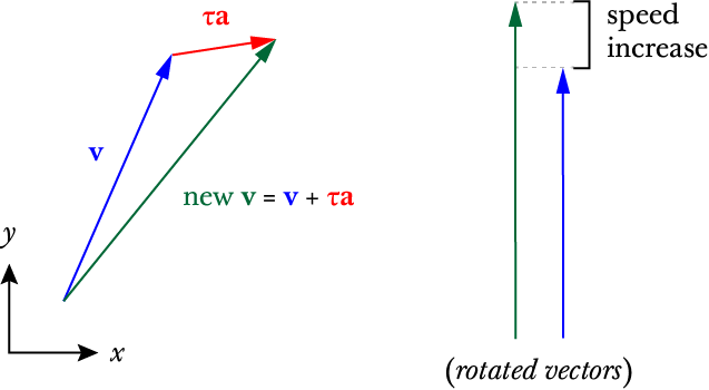
Fig. 6.1. Depiction of how strafing increases speed (i.e. the length of the velocity vector). On the left, the directions of the vectors have significance. On the right, we have rotated the vectors to that they line up, but therefore do not point to the correct direction (though having the correct length or magnitude).

In Half-Life physics, the magnitude or length of the acceleration vector 𝐚 depends on the current speed and the angle between the velocity and itself, which in turn is controlled by the viewangles, as explained in Air and ground movements. The task of finding the optimal angles to achieve a certain goal is the topic of this chapter.

6.2. Building blocks

Regardless of the objective of strafing, its physics is governed by the fundamental movement equation (FME). We will construct several few mathematical building blocks to aid further analyses. Firstly, write ‖𝐯′‖ =√𝐯′⋅𝐯′, where 𝐯′ is already given in Air and ground movements. Expanding each 𝐯′ yields

(6.1)‖𝐯′‖=√(𝜆(𝐯)+𝜇ˆ𝐚)⋅(𝜆(𝐯)+𝜇ˆ𝐚)=√‖𝜆(𝐯)‖2+𝜇2+2‖𝜆(𝐯)‖𝜇cos⁡𝜃

This can be done because the dot product satisfies the distributive law. Very quickly, we obtained (6.1) which is sometimes called the scalar FME, often used in practical applications as the most general way to compute new speeds (as opposed to velocity vectors) given 𝜃.

Tip

This is a very common and useful trick that can be used to quickly yield an expression for the magnitude of vectorial outputs without explicit vectorial computations or geometric analyses. Half-Life physicists ought to learn this technique well.

From equation (6.1), we can further write down the equations by assuming 𝜇 =𝛾1 and 𝜇 =𝛾2 respectively, to eliminate 𝜇. These new equations can be found by expanding 𝜇, again already given previously. We get

(6.2)‖𝐯′𝜇=𝛾1‖=√‖𝜆(𝐯)‖2+𝑘𝑒𝜏𝑀𝐴(𝑘𝑒𝜏𝑀𝐴+2‖𝜆(𝐯)‖cos⁡𝜃)‖𝐯′𝜇=𝛾2‖=√‖𝜆(𝐯)‖2sin2⁡𝜃+𝐿2

Note that when 𝛾1 =𝛾2, we have ‖𝐯′𝜇=𝛾1‖ =‖𝐯′𝜇=𝛾2‖. Define 𝜁 such that

cos⁡𝜁=𝐿−𝑘𝑒𝜏𝑀𝐴‖𝜆(𝐯)‖

Assuming 𝛾2 ≥0, then if cos⁡𝜃 ≤cos⁡𝜁, we have 𝜇 =𝛾1. If cos⁡𝜃 ≥cos⁡𝜁, then 𝜇 =𝛾2. Define also ¯𝜁 such that 𝛾2 <0 and therefore 𝜇 =0, as

cos⁡¯𝜁=𝐿‖𝜆(𝐯)‖

Note

Note that we permit |cos⁡𝜁| >1 and |cos⁡¯𝜁| >1, but restricts |cos⁡𝜃| ≤1. We never need to invert the cosines to obtain 𝜁 and ¯𝜁 in theoretical and practical computations when their absolute values are greater than 1. However, had we really done it, 𝜁 and ¯𝜁 would have imaginary parts.

Putting these together, we can write the 𝜇 more explicitly as a piecewise-defined function

(6.3)𝜇=⎧{ {⎨{ {⎩0cos⁡𝜃≥cos⁡¯𝜁𝛾2cos⁡𝜃<cos⁡¯𝜁∧cos⁡𝜃≥cos⁡𝜁𝛾1cos⁡𝜃<cos⁡¯𝜁∧cos⁡𝜃≤cos⁡𝜁

The new speed ‖𝐯′‖ can also be correspondingly written as a piecewise-defined function by substituting 𝜇 with (6.3). These equations will be important in the exploitative analyses of the FME shortly.

However, computing speeds is sometimes not sufficient. We sometimes want to also compute velocity vectors endowed with both directionality and magnitude, but without worrying about player viewangles and ˆ𝐚. We can achieve this by parametrising ˆ𝐚 in terms of a rotation of ˆ𝐯 by an angle of 𝜃. This may be expressed as

ˆ𝐚=ˆ𝐯𝑅𝑧(𝜃)

This is a matrix multiplication of ˆ𝐯 by a rotation matrix. The benefit of writing the FME in this form is that we no longer need to worry about calculating ˆ𝐟 and ˆ𝐬, which, recalling from View vectors, depend on the yaw angle 𝜗 in the 2D case. We also no longer need to worry about 𝐹, 𝑆, and 𝑀 needed to compute ˆ𝐚. All we need to know is the angle 𝜃 between velocity and acceleration vectors. This can make efficient computations easier as well, because the angle 𝜃 is easily computed (as we will see shortly) in just a few lines of code.

Caution

Remember from Notations Used that vectors in this documentation are row vectors. Therefore, the order of multiplication is different from those in standard linear algebra textbooks. In fact, the components in 𝑅𝑧(𝜃) are also ordered differently.

With this idea in mind, we can rewrite the FME as

(6.4)𝐯′=𝜆(𝐯)+𝜇ˆ𝐯[cos⁡𝜃−sin⁡𝜃sin⁡𝜃cos⁡𝜃](𝐯≠𝟎)

Note that the precaution 𝐯 ≠𝟎 is needed so that the unit vector ˆ𝐯 =𝐯/‖𝐯‖ is well defined. In other words, the directionality of 𝐯 is lost when it is zero. This is therefore one downside of parametrising in terms of 𝜃, where the special case of zero velocity must be handled separately by replacing ˆ𝐯 =ˆ𝐟 (and assuming 𝜑 =0 as usual) in (6.4), thereby involving the viewangles in the computations.

When written in the form of (6.4), positive 𝜃 gives clockwise rotations, while negative 𝜃 gives anticlockwise rotations. If this convention is inconvenient for a particular application, one can easily reverse the directionality by reversing the signs of the sin⁡𝜃 elements in the rotation matrix.

6.3. Maximum acceleration

Airstrafing to continuously gain speed beyond what the developers intended is one of the oldest speedrunning tricks. It is of no surprise that one of the earliest inquiries into Half-Life physics is related to the question of how to airstrafe with the maximum acceleration, when research began circa 2012 by the author of this documentation. In this section, we will provide precise mathematical descriptions of how maximum-acceleration strafing works in a way that will provide a baseline for further analyses and also can readily be implemented in TAS tools.

We must define our metric for “maximum acceleration” in a mathematically precise way. Specifically, we want to maximise the average scalar acceleration over some period of time 𝑡. The average scalar acceleration may in turn be defined as

―――‖𝐚‖=Δ‖𝐯‖𝑡=‖𝐯𝑡‖−‖𝐯0‖𝑡

where ‖𝐯𝑡‖ is the speed at time 𝑡 and ‖𝐯0‖ is the initial speed. We believe this is a valid metric because it reflects the intention of the speedrunner better in the field: namely, to increase the speed as much as possible over some time, which automatically also increases the distance travelled within the same period of time, since the distance travelled is simply the sum of all the speeds in every frame within the period of time in question.

6.3.1. Arguments of the maxima

Let 𝐯 be the current player velocity, 𝐯′ the velocity after strafing, and 𝜏𝑔 the game frame time (see Frame rate). To maximise the average scalar acceleration, it is sufficient to maximise the per-frame scalar acceleration

‖𝐯′‖−‖𝐯‖𝜏𝑔

It turns out that maximising the per-frame acceleration “greedily” also maximises the global average acceleration over the span of some time 𝑡. In other words, optimising only the individual frames result in the optimal “overall” acceleration as well. This is perhaps owing to good luck, because it is by no means a universal rule that local maxima yield a global maximum in other instances. We will prove this assertion in a later section.

Now, we will assume ‖𝐯‖ and 𝜏𝑔 are independent of any other variables. Therefore, we can ignore them, and the task of maximising acceleration boils down to maximising solely the new speed ‖𝐯′‖. Looking at (6.2), observe that the new speed is invariant to the transformation 𝜃 ↦ −𝜃, because both cos⁡𝜃 and sin2⁡𝜃 are even functions. Without loss of generality, we will consider only 0 ≤𝜃 ≤𝜋.

Before we search for the global optimum, we must understand the behaviours of the piecewise ‖𝐯′‖. Observe that the maximum of ‖𝐯′𝜇=𝛾2‖ occurs at sin⁡𝜃 =1 or cos⁡𝜃 =0, if we consider the entire domain of −1 ≤cos⁡𝜃 ≤1, or

argmaxcos⁡𝜃‖𝐯′𝜇=𝛾2‖=0

In addition, we also see that ‖𝐯′𝜇=𝛾2‖ is strictly increasing in −1 ≤cos⁡𝜃 ≤0 and strictly decreasing in 0 ≤cos⁡𝜃 ≤1. Indeed, the plot for ‖𝐯′𝜇=𝛾2‖ against cos⁡𝜃 forms a semi-ellipse except in degenerate cases.

On the other hand, the maximum of ‖𝐯′𝜇=𝛾1‖, however, depends on the sign of 𝑘𝑒𝜏𝑀𝐴. The symbols here have already been defined in Air and ground movements.

argmaxcos⁡𝜃‖𝐯′𝜇=𝛾1‖=⎧{ {⎨{ {⎩1𝑘𝑒𝜏𝑀𝐴>0−1𝑘𝑒𝜏𝑀𝐴<0[−1,1]𝑘𝑒𝜏𝑀𝐴=0

If 𝑘𝑒𝜏𝑀𝐴 >0, then ‖𝐯′𝜇=𝛾1‖ is strictly increasing. If 𝑘𝑒𝜏𝑀𝐴 <0, then ‖𝐯′𝜇=𝛾1‖ is strictly decreasing.

The relative sizes of {0,cos⁡𝜁,cos⁡¯𝜁} can vary in various ways, and there are in total 3! =6 permutations we must consider in order to study the behaviour of the new speed ‖𝐯′‖ and therefore the maximum point.

0 ≤cos⁡𝜁 ≤cos⁡¯𝜁

If and only if 𝐿 −𝑘𝑒𝜏𝑀𝐴 ≥0, 𝐿 ≥0, and 𝑘𝑒𝜏𝑀𝐴 ≥0. In −1 ≤cos⁡𝜃 ≤cos⁡𝜁, ‖𝐯′‖ =‖𝐯′𝜇=𝛾1‖ is strictly increasing with a maximum point at cos⁡𝜃 =cos⁡𝜁. In cos⁡𝜁 ≤cos⁡𝜃 ≤cos⁡¯𝜁, ‖𝐯′‖ =‖𝐯′𝜇=𝛾2‖ is strictly decreasing. However, if cos⁡𝜁 >1, then 𝜇 =𝛾1 for the entire range. We conclude that

argmaxcos⁡𝜃‖𝐯′‖=min(1,cos⁡𝜁),𝜇=𝛾1

0 ≤cos⁡¯𝜁 ≤cos⁡𝜁

If and only if 𝐿 −𝑘𝑒𝜏𝑀𝐴 ≥0, 𝐿 ≥0, and 𝑘𝑒𝜏𝑀𝐴 ≤0. In −1 ≤cos⁡𝜃 ≤cos⁡¯𝜁, ‖𝐯′‖ =‖𝐯′𝜇=𝛾1‖ is strictly decreasing with a maximum point at cos⁡𝜃 = −1. In cos⁡¯𝜁 ≤cos⁡𝜃 ≤cos⁡𝜁, ‖𝐯′‖ =‖𝜆(𝐯)‖. Therefore, we always have

argmaxcos⁡𝜃‖𝐯′‖=−1,𝜇=𝛾1

cos⁡𝜁 ≤0 ≤cos⁡¯𝜁

If and only if 𝐿 −𝑘𝑒𝜏𝑀𝐴 ≤0, 𝐿 ≥0, and 𝑘𝑒𝜏𝑀𝐴 ≥0. In −1 ≤cos⁡𝜃 ≤cos⁡𝜁, ‖𝐯′‖ =‖𝐯′𝜇=𝛾1‖ is strictly increasing. In cos⁡𝜁 ≤cos⁡𝜃 ≤cos⁡¯𝜁, the maximum occurs at cos⁡𝜁 =0. This implies

argmaxcos⁡𝜃‖𝐯′‖=0,𝜇=𝛾2

cos⁡¯𝜁 ≤0 ≤cos⁡𝜁

If and only if 𝐿 −𝑘𝑒𝜏𝑀𝐴 ≥0, 𝐿 ≤0, and 𝑘𝑒𝜏𝑀𝐴 ≤0. In −1 ≤cos⁡𝜃 ≤cos⁡¯𝜁 ≤cos⁡𝜁, we have ‖𝐯′‖ =‖𝐯′𝜇=𝛾1‖, which is strictly decreasing because 𝑘𝑒𝜏𝑀𝐴 ≤0. Therefore, the maximum point is at

argmaxcos⁡𝜃‖𝐯′‖={−1cos⁡¯𝜁>−1[−1,1]cos⁡¯𝜁≤−1𝜇=𝛾1

cos⁡𝜁 ≤cos⁡¯𝜁 ≤0

If and only if 𝐿 −𝑘𝑒𝜏𝑀𝐴 ≤0, 𝐿 ≤0, and 𝑘𝑒𝜏𝑀𝐴 ≥0. In −1 ≤cos⁡𝜃 ≤cos⁡𝜁, ‖𝐯′‖ =‖𝐯′𝜇=𝛾1‖ is strictly increasing. In cos⁡𝜁 ≤cos⁡𝜃 ≤cos⁡¯𝜁 ≤0, ‖𝐯′‖ =‖𝐯𝜇=𝛾2‖ is also strictly increasing. But since ‖𝐯′𝜇=𝛾2‖ =0 at cos⁡𝜃 =cos⁡¯𝜁, we conclude that

argmaxcos⁡𝜃‖𝐯′‖=[max(−1,cos⁡¯𝜁),1],𝜇=0

As we will see later, this case actually yields ‖𝐯′‖ =‖𝐯‖, which is useless. But we will include this case for the sake of completeness.

cos⁡¯𝜁 ≤cos⁡𝜁 ≤0

If and only if 𝐿 −𝑘𝑒𝜏𝑀𝐴 ≤0, 𝐿 ≤0, 𝑘𝑒𝜏𝑀𝐴 ≤0. The rest of the analysis and the result are exactly the same as that in the cos⁡¯𝜁 ≤0 ≤cos⁡𝜁 case.

Given the case-by-case study of these six permutations, we can summarise that the maximum point of ‖𝐯′‖ occurs at

(6.5)cos⁡𝜃=cos⁡Θ∈argmaxcos⁡𝜃‖𝐯′‖=⎧{ { { {⎨{ { { {⎩min(1,cos⁡𝜁)𝑘𝑒𝜏𝑀𝐴≥0∧𝐿−𝑘𝑒𝜏𝑀𝐴≥0∧𝐿≥00𝑘𝑒𝜏𝑀𝐴≥0∧𝐿−𝑘𝑒𝜏𝑀𝐴≤0∧𝐿≥0[max(−1,cos⁡¯𝜁),1]𝑘𝑒𝜏𝑀𝐴≥0∧𝐿−𝑘𝑒𝜏𝑀𝐴≤0∧𝐿≤0[−1,1]𝑘𝑒𝜏𝑀𝐴≤0∧cos⁡¯𝜁≤−1−1𝑘𝑒𝜏𝑀𝐴≤0∧cos⁡¯𝜁>−1

To implement (6.5), care must be taken when computing cos⁡𝜁 and cos⁡¯𝜁. This is because when ‖𝜆(𝐯)‖ =0, we have cos⁡𝜁 = ±∞ and cos⁡¯𝜁 = ±∞.

6.3.2. Optimality

We show that the angles given in (6.5) actually gives the highest average acceleration over some time 𝑡, more than just the maximum speed after one frame of strafing. After one frame of strafing, the average acceleration is given by

‖𝐯1‖−‖𝐯0‖𝜏𝑔

Since the only variable is ‖𝐯1‖, clearly the angles in (6.5) maximises the acceleration. Now suppose the player has strafed for some time 𝑡 at a maximum average acceleration possible ¯𝑎 so that the final speed is some ‖𝐯𝑛‖ =¯𝑎𝑡, and it is required to strafe another frame. The new average acceleration after another frame is then

‖𝐯𝑛+1‖−‖𝐯0‖𝑡+𝜏𝑔

where ‖𝐯𝑛+1‖ is given by the FME with ‖𝐯𝑛‖ as the starting speed. Since the only variable is again ‖𝐯𝑛+1‖, clearly (6.5) gives the maximum ‖𝐯𝑛+1‖. We conclude by induction that (6.5) gives the maximum average acceleration over some time 𝑡.

On top of that, we also show that (6.5) gives the highest average speed over some time 𝑡. In other words, it admits the shortest time possible to travel any distance 𝑑. Given an initial speed of ‖𝐯0‖, the average speed after one frame of strafing is

‖𝐯1‖𝜏𝜏𝑔

Clearly (6.5) gives the maximum average speed because ‖𝐯1‖ is the only variable. Now, suppose the player has strafed for some time 𝑡 at the maximum possible average speed ¯𝑣 with some final speed ‖𝐯𝑛‖. After another frame of strafing, the new average speed is

¯𝑣𝑡+‖𝐯𝑛+1‖𝜏𝑡+𝜏𝑔

where ‖𝐯𝑛+1‖ is given by the FME with ‖𝐯𝑛‖ as the starting speed and is the only variable. Again, the angles given by (6.5) maximises ‖𝐯𝑛+1‖.

6.3.3. Speed equations

Using (6.5) we obtain the optimal cos⁡𝜃 under various situations. We can proceed to eliminate 𝜃 and 𝜇 from (6.1) to obtain a clean formulae for speed after one frame. Further, we can also obtain formulae for the speed after 𝑛 frames, assuming all the movement variables are held constant.

(6.6)‖𝐯′‖=⎧{ { { {⎨{ { { {⎩√‖𝜆(𝐯)‖2+𝑘𝑒𝜏𝑀𝐴(2𝐿−𝑘𝑒𝜏𝑀𝐴)case 1∧cos⁡Θ=cos⁡𝜁‖𝜆(𝐯)‖+𝑘𝑒𝜏𝑀𝐴case 1∧cos⁡Θ=1√‖𝜆(𝐯)‖2+𝐿2case 2‖𝜆(𝐯)‖case 3 & 4‖𝜆(𝐯)‖−𝑘𝑒𝜏𝑀𝐴case 5

For airstrafing where there is no friction (namely 𝜆(𝐯) =𝐯), we can solve the recurrence relations easily and obtain formulae for the speed after 𝑛 frames of strafing as follows:

(6.7)‖𝐯𝑛‖=⎧{ { { {⎨{ { { {⎩√‖𝐯0‖2+𝑛𝑘𝑒𝜏𝑀𝐴(2𝐿−𝑘𝑒𝜏𝑀𝐴)case 1∧cos⁡Θ=cos⁡𝜁‖𝐯0‖+𝑛𝑘𝑒𝜏𝑀𝐴case 1∧cos⁡Θ=1√‖𝐯0‖2+𝑛𝐿2case 2‖𝐯0‖case 3 & 4‖𝐯0‖−𝑛𝑘𝑒𝜏𝑀𝐴case 5

These equations can be quite useful in planning. For example, to calculate the number of frames required to airstrafe from 320 ups to 1000 ups at default Half-Life settings and 1000 fps, we solve

10002=3202+𝑛⋅0.001⋅320⋅10⋅(60−0.001⋅320⋅10)⟹𝑛≈4938

In addition, under airstrafing again, we can integrate the speed equations to obtain distance-time equations. Before doing this, we must make a change of variables by assuming continuous time and writing 𝑡 =𝑛𝜏. Then we compute

𝑑𝑡=∫𝑡0‖𝐯𝑡′‖𝑑𝑡′

for each case.

For groundstrafing, however, the presence of friction means simple substitutions may not work. In more complex cases, it may be desirable to simply calculate the speeds frame by frame using the scalar FME.

6.3.4. Effects of frame rate

The frame rate can affect the acceleration significantly. Looking at the second case of (6.5), the acceleration per frame is

√‖𝜆(𝐯)‖2+𝐿2−‖𝜆(𝐯)‖𝜏𝑔

One can immediately see that the lower the 𝜏𝑔 (that is, the higher the game frame rate), the higher the acceleration. The first case of (6.5) and cos⁡Θ =cos⁡𝜁 also provides greater accelerations at greater game frame rates. The other cases, however, do not admit greater accelerations at higher frame rates.

6.3.4.1. When 𝜂 ≠1

Recall in Frame rate that, on older game engines, the player frame rate 𝜏𝑝 is the game frame rate rounded towards zero to the nearest 0.001. This is not normally a problem, because speedruns are often run at frame rates such that 𝜏𝑝 =𝜏𝑔, thus eliminating any slowdown. However, at the time of writing (July 2020), there exists an area of contention regarding the WON version of Blue Shift, where the default frame rate is 72 fps and some community rules forbid raising it further via console commands. Clearly, the slowdown factor at 72 fps is less than 1. There is a question of whether it is optimal to

1. use a lower 𝜏𝑔 such that 𝜏𝑝 =𝜏𝑔 (which would be 𝜏𝑔 =0.014 or 𝑓𝑔 ≈71.43 in the WON Blue Shift case), or

2. use 𝜏𝑔 =1/72 and 𝜏𝑝 =0.013 in some of the frames and switch to 𝜏𝑝 =𝜏𝑔 =0.014 in other frames

We claim that it is better to always lower 𝜏𝑔 such that 𝜏𝑝 =𝜏𝑔 and 𝜂 =1. Precisely, we claim that the average speed over some real time 𝑡 is maximised when 𝜂 =1 throughout time 𝑡. To see why, recall that the average speed is simply the total distance travelled divided by the time taken. The average speed in the first frame is

𝑉1=𝜏𝑝,1√‖𝐯0‖2+𝐾2𝜏𝑔,1=𝜂1√‖𝐯0‖2+𝐾2

Immediately, we can see that to maximise the average speed, we must have 𝜏𝑝,1 =𝜏𝑔,1 so that 𝜂 =1 is as big as possible. Now suppose the player has already travelled for some distance at a maximum average speed 𝑉𝑛, taking some real time 𝑡. We need to strafe another frame. The new average speed is then given by

𝑉𝑛+1=𝑡𝑉𝑛+𝜏𝑝,𝑛+1‖𝐯𝑛+1‖𝑡+𝜏𝑔,𝑛+1

Recall that 𝜏𝑝,𝑛+1 =1000−1⌊1000𝜏𝑔,𝑛+1⌋. Write 𝜏𝑔,𝑛+1 =𝜏𝑝,𝑛+1 +𝜖 for some 0 ≤𝜖 <0.001. Eliminating 𝜏𝑔,𝑛+1, the new average speed may be rewritten as

𝑉𝑛+1=𝑡𝑉𝑛+𝜏𝑝,𝑛+1‖𝐯𝑛+1‖𝑡+𝜏𝑝,𝑛+1+𝜖

Observe that to maximise 𝑉𝑛+1, we must have 𝜖 =0 which implies 𝜏𝑔,𝑛+1 =𝜏𝑝,𝑛+1. By induction, we have proved our claim stated earlier.

6.3.5. Effects of friction

There is a limit to the speed achievable by maximum-acceleration groundstrafing alone. There will be a critical speed such that the increase in speed exactly cancels the friction, so that ‖𝐯𝑘+1‖ =‖𝐯𝑘‖, namely the speed reaches a steady state. For the common example of default game settings, suppose the cos⁡Θ =cos⁡𝜁 (the first case of (6.6)), 𝐿 =𝑀 (see Air and ground movements), and geometric friction (see Ground friction) is at play. Then we may write

‖𝐯‖2=(1−𝜏𝑘)2‖𝐯‖2+𝑘𝑒𝜏𝑀2𝐴(2−𝑘𝑒𝜏𝐴)

Solving for ‖𝐯‖, we obtain the maximum groundstrafe speed for this particular configuration, keeping in mind that 𝑘 is dependent on 𝑘𝑒:

𝑀√𝑘𝑒𝐴(2−𝜏𝑘𝑒𝐴)𝑘(2−𝜏𝑘)

Take the case of default Half-Life settings at 1000 fps, we calculate

320√1⋅10⋅(2−0.001⋅1⋅10)4⋅(2−0.001⋅4)≈505.2

This is then the absolute maximum speed achievable by groundstrafing alone in vanilla Half-Life. At another common frame rate of 100 fps, we instead obtain the steady state speed of ≈498.2. There is nothing we can do to groundstrafe beyond this speed!

Interestingly, when there is edge friction, the game sets 𝑘 =8 with the default settings, and the maximum groundstrafe speed is drastically reduced to ≈357.6, which is indeed devastating as previously claimed in Edgefriction, because it is not significantly more than the normal running speed of 320.

We also see that when the entity friction 𝑘𝑒 is less than 1, the effect on the maximum groundstrafe speed is very small. For instance, if 𝑘𝑒 =0.5, then 𝑘 =2. This yields the maximum groundstrafe speed of ≈505.6, barely larger than the normal groundstrafe speed.

Traditionally, jumping is done repeatedly to lift off from the ground to avoid the effects of ground friction. However, the presence of the bunnyhop cap (see Bunnyhop cap) compels speedrunners to opt for ducktapping (see Ducktapping) instead. Ducktapping has a downside of requiring one frame of ground contact, which introduces one frame of friction. The effect of this one frame of friction can be completely eliminated by setting the frame rate to an extremely high value in that frame alone, which forces 𝜏𝑝 =0 while the player is on the ground. If this is not possible, or forbidden, then the one frame of friction is unavoidable.

It turns out that the single frame of ground friction can be devastating, especially in lower frame rates. In fact, under most circumstances and combinations of movement variables, there exists a fixed point or steady state speed which acts as a limit to the speed a player can maintain indefinitely using only ducktapping and strafing alone. Let ‖𝐯‖𝑆 be this steady state speed. Let MaxAccel⁡(type,𝑣0,𝑛) be a function that gives the speed after 𝑛 frames of maximum-acceleration strafing from an initial speed of 𝑣0. Denote 𝑇𝐷 the ducktap “period”, or the time the player spends in the air after a ducktap. Define functions

𝑉𝐴(𝑣0):=MaxAccel⁡(air,𝑣0,𝑇𝐷𝜏−1)𝑉𝐺(𝑣0):=MaxAccel⁡(ground,𝜆(𝑉𝐴(𝑣0)),1)

Then 𝑉𝐺 gives the speed when the player lands on the ground after a ducktap and airstrafing. In general, to find the steady state speed ‖𝐯‖𝑆, we solve the equation

(6.8)𝑉𝐺(‖𝐯‖𝑆)=‖𝐯‖𝑆

To give some concrete examples, consider ducktapping and strafing in a typical 1000 fps TAS with default Half-Life settings. Assuming ‖𝐯‖𝑆 >𝐸 so that the geometric friction is in effect. Then (6.8) can be rewritten using (6.6) and (4.2) as

√(‖𝐯‖2𝑆+𝑇𝐷𝐶𝐴)(1−𝑘𝜏)2+𝐶𝐺=‖𝐯‖𝑆

where

𝐶𝐴=𝑘𝑒𝑀𝐴𝐴(60−𝑘𝑒𝜏𝑀𝐴𝐴),𝐶𝐺=𝑘𝑒𝜏𝑀2𝐴𝐺(2−𝑘𝑒𝜏𝐴𝐺)

Assuming 𝑇𝐷 =0.2, we obtain ‖𝐯‖𝑆 ≈2184. This implies that the player is able to maintain at least the default sv_maxvelocity at 1000 fps by ducktapping and strafing. Consider, however, ducktapping and strafing at 100 fps, which is a restriction some in the community are in favour of imposing. Here, (6.8) may instead be rewritten as

√(‖𝐯‖2𝑆+𝑇𝐷𝜏−1900)(1−𝑘𝜏)2+𝐶𝐺=‖𝐯‖𝑆

With 𝜏 =0.01 and solving, we instead obtain ‖𝐯‖𝑆 ≈678, which is substantially lower than that at 1000 fps.

6.3.6. Growth of speed

By obtaining (6.7), we can immediately make a few important observations. In the absence of friction and if |cos⁡Θ| ≠1, the speed over time grows sublinearly, or 𝑂(√𝑛). This implies that the acceleration gradually decreases over time, but never reaches zero. It is notable that the acceleration at lower speeds can be substantial (more than linear acceleration) compared to that at higher speeds. To see why, write new speed 𝑣𝑡 =√𝑣20+𝑡𝐾, then taking the derivative with respective to 𝑡 to obtain acceleration, yielding

𝑎𝑡=𝑑𝑣𝑡𝑑𝑡=𝐾2√𝑣20+𝑡𝐾

for some 𝐾. Now observe that, at 𝑡 =0, the acceleration 𝑎𝑡 →∞ as initial speed decreases 𝑣0 →0.

When |cos⁡Θ| =1, however, possibly in the first case and the fifth case of (6.5), the growth of speed is linear. Even with the presence of ground friction, the growth of speed can be linear under an arithmetic friction. For example, in the default game settings, cos⁡Θ =1 on the ground when ‖𝐯‖ ≤𝑀(1−𝑘𝑒𝜏𝐴). In addition, the arithmetic friction is at play when ‖𝐯‖ <𝐸. Therefore, the speed at the 𝑛-th frame is

‖𝐯𝑛‖=‖𝐯0‖+𝑛𝜏(𝑘𝑒𝑀𝐴−𝐸𝑘)

as long as ‖𝐯𝑛‖ <min(𝐸,𝑀(1−𝑘𝑒𝜏𝐴)).

6.3.7. Air-ground speed threshold

The acceleration of groundstrafe is usually greater than that of airstrafe. It is for this reason that groundstrafing is used to initiate bunnyhopping. However, once the speed increases beyond 𝐸 the acceleration will begin to decrease, as the friction grows proportionally with the speed. There will be a critical speed beyond which the acceleration of airstrafe exceeds that of groundstrafe. This is called the air-ground speed threshold (AGST), admittedly a rather non-descriptive name.

Fig. 6.2. Comparison between the accelerations arising from strafing in the air and on the ground at various speeds at default Half-Life settings and 1000 fps. Although the acceleration in the air is greater than that on the ground when the speed is very low, the acceleration in the air rapidly falls as speed increases. The air and ground accelerations cross later at the air-ground speed threshold of approximately 482 ups.

Analytic solutions for AGST are always available, but they are cumbersome to write and code. Sometimes the speed curves for airstrafe and groundstrafe intersects several times, depending even on the initial speed itself. A more practical solution in practice is to simply use Equation (6.1) to compute the new airstrafe and groundstrafe speeds then comparing them.

It is also important to note that, even if the air acceleration is greater than the ground acceleration for a given speed, it does not mean that it is optimal to actually leave the ground for air acceleration at that particular time. To illustrate, assume the default Half-Life settings and 𝜏 =0.001. Suppose also the player is on the ground, and the speed is very low at ‖𝐯‖ =30. After one frame of groundstrafing, the new speed would be

‖𝐯′ground‖=‖𝐯‖+𝜏(𝑘𝑒𝑀𝐴−𝐸𝑘)=30+0.001⋅(1⋅320⋅10−100⋅4)=32.8

On the other hand, the player could also ducktap or jump to get into the air and airstrafe, which would have yielded a speed of

‖𝐯′air‖=√‖𝐯‖2+𝑘𝑒𝜏𝑀𝐴(2𝐿−𝑘𝑒𝜏𝑀𝐴)=√302+1⋅0.001⋅320⋅10(60−1⋅0.001⋅320⋅10)≈32.89

We have ‖𝐯′air‖ >‖𝐯′ground‖. If the player actually ducktaps to leave the ground, it would have taken the player approximately 0.25s to land back onto the ground. However, before the player could have done so, the air acceleration would have already diminished owing to the sublinear growth mentioned in Growth of speed. For example, even with ‖𝐯‖ =40, the next speed is ≈42.2 for a speed difference of ≈2.2, which is lower than what would be obtained from groundstrafing.

6.3.8. Effects of bunnyhop cap

It is impossible to avoid the bunnyhop cap (see Bunnyhop cap) when jumping in later official releases of the game. To lift off the ground and avoid the effects of ground friction, one alternative would be to ducktap instead (see Ducktapping). However, each ducktap requires the player to slide on the ground for one frame. Without using very high frame rates to force the frame to be 𝜏𝑝 =0, the player will lose speed due to friction, especially at lower frame rates. In addition, the player cannot ducktap if there is insufficient clearance above the player. In such cases, jumping is the only way to maintain speed, though there are different possible ways to approach this. Regardless of the movement strategy, we must not trigger the cap itself when jumping, because that would cause an instant and significant reduction in speed.

It turns out that the answer is not as straightforward as we may have thought and would require more investigations.

6.4. Maximum deceleration

It is often the case that the player needs to rapidly decelerate in the air or on the ground without any aid using weapons, damage, or solid entities. When the player is on the ground, deceleration is easy to achieve by simply issuing the +use command, which would exponentially reduce the velocity by a factor of 0.3 per frame. When the player is in the air, however, the player must rely on the pure air movement physics to decelerate as much as possible.

6.4.1. Arguments of the minima

Using the tools and partial results we built earlier in Maximum acceleration, we can perform a similar case-by-case analysis for the different permutations of {0,cos⁡𝜁,cos⁡¯𝜁}. We will not repeat some of the steps in the following analyses.

0 ≤cos⁡𝜁 ≤cos⁡¯𝜁

If cos⁡𝜁 ≥1, then the minimum point is simply at cos⁡𝜃 = −1 since 𝜇 =𝛾1 for all −1 ≤cos⁡𝜃 ≤1.

Suppose cos⁡𝜁 <1 and cos⁡¯𝜁 >1. Then, ‖𝐯′‖ =‖𝐯′𝜇=𝛾2‖ is strictly decreasing in cos⁡𝜁 ≤cos⁡𝜃 ≤1, so we must consider the points cos⁡𝜃 = ±1. We show that the global minimum is still at cos⁡𝜃 = −1. Calculate the local minima at cos⁡𝜃 = −1 and cos⁡𝜃 =1:

‖𝐯′(cos⁡𝜃=−1)‖=∣‖𝜆(𝐯)‖−𝑘𝑒𝜏𝑀𝐴∣‖𝐯′(cos⁡𝜃=1)‖=𝐿

Suppose the minimum point is at cos⁡𝜃 =1. This implies

‖𝐯′(cos⁡𝜃=1)‖≤‖𝐯′(cos⁡𝜃=−1)‖𝐿≤∣‖𝜆(𝐯)‖−𝑘𝑒𝜏𝑀𝐴∣

Assume ‖𝜆(𝐯)‖ −𝑘𝑒𝜏𝑀𝐴 ≥0. Then this implies

𝐿+𝑘𝑒𝜏𝑀𝐴≤‖𝜆(𝐯)‖

which is a contradiction, because our supposition that cos⁡¯𝜁 >1 implies ‖𝜆(𝐯)‖ <𝐿. Assume instead that ‖𝜆(𝐯)‖ −𝑘𝑒𝜏𝑀𝐴 ≤0. Then we obtain

−(𝐿−𝑘𝑒𝜏𝑀𝐴)≥‖𝜆(𝐯)‖

But 0 ≤cos⁡𝜁 implies 𝐿 −𝑘𝑒𝜏𝑀𝐴 ≥0 and clearly ‖𝜆(𝐯)‖ ≥0, which is a contradiction. This concludes the proof.

Suppose cos⁡𝜁 ≤cos⁡¯𝜁 ≤1. Then in −1 ≤cos⁡𝜃 ≤cos⁡𝜁, ‖𝐯′‖ =‖𝐯′𝜇=𝛾1‖ is strictly increasing with a minimum point at cos⁡𝜃 = −1. In cos⁡𝜁 ≤cos⁡𝜃 ≤cos⁡¯𝜁, ‖𝐯′‖ =‖𝐯′𝜇=𝛾2‖ is strictly decreasing with a minimum point at cos⁡𝜃 =cos⁡¯𝜁 and a minimum value of ‖𝐯′‖ =‖𝜆(𝐯)‖ corresponding to 𝜇 =0. In cos⁡¯𝜁 ≤cos⁡𝜃 ≤1, the value stays at ‖𝐯′‖ =‖𝜆(𝐯)‖. We show that the global minimum is yet again at cos⁡𝜃 = −1. Calculate the local minima corresponding to cos⁡𝜃 = −1 and cos⁡𝜃 ∈[cos⁡¯𝜁,1]. We have

‖𝐯′(cos⁡𝜃=−1)‖=∣‖𝜆(𝐯)‖−𝑘𝑒𝜏𝑀𝐴∣‖𝐯′(cos⁡𝜃∈[cos⁡¯𝜁,1])‖=‖𝜆(𝐯)‖

Suppose the global minimum is at cos⁡𝜃 ∈[cos⁡¯𝜁,1]. This implies

‖𝜆(𝐯)‖≤∣‖𝜆(𝐯)‖−𝑘𝑒𝜏𝑀𝐴∣

Assume ‖𝜆(𝐯)‖ −𝑘𝑒𝜏𝑀𝐴 ≥0. Then we obtain

0≥𝑘𝑒𝜏𝑀𝐴

which is a contradiction. Assume instead that ‖𝜆(𝐯)‖ −𝑘𝑒𝜏𝑀𝐴 ≤0, which implies

‖𝜆(𝐯)‖≤12𝑘𝑒𝜏𝑀𝐴

But cos⁡¯𝜁 ≤1 implies 𝐿 ≤‖𝜆(𝐯)‖. Putting these inequalities together yields

𝐿−12𝑘𝑒𝜏𝑀𝐴≤0

Since 𝐿 ≥0 and 𝑘𝑒𝜏𝑀𝐴 ≥0, this further implies that

𝐿−𝑘𝑒𝜏𝑀𝐴<𝐿−12𝑘𝑒𝜏𝑀𝐴≤0

But 0 ≤cos⁡𝜁 implies 𝐿 −𝑘𝑒𝜏𝑀𝐴 ≥0, which is a contradiction. This concludes the proof.

We conclude that

argmincos⁡𝜃‖𝐯′‖=−1

0 ≤cos⁡¯𝜁 ≤cos⁡𝜁

In −1 ≤cos⁡𝜃 ≤cos⁡¯𝜁, ‖𝐯′‖ =‖𝐯′𝜇=𝛾1‖ is strictly decreasing. In cos⁡¯𝜁 ≤cos⁡𝜃 ≤1, we have ‖𝐯′‖ =‖𝜆(𝐯)‖. If cos⁡¯𝜁 >1, the minimum point is at cos⁡𝜃 =1 because ‖𝐯′𝜇=𝛾1‖ is strictly decreasing. We conclude that

argmincos⁡𝜃‖𝐯′‖=[min(1,cos⁡¯𝜁),1]

cos⁡𝜁 ≤0 ≤cos⁡¯𝜁

Suppose cos⁡𝜁 < −1 and cos⁡¯𝜁 >1. Then ‖𝐯′‖ =‖𝐯′𝜇=𝛾2‖ for all −1 ≤cos⁡𝜃 ≤1. Since ‖𝐯′𝜇=𝛾2 is an even function in cos⁡𝜃, we have

argmincos⁡𝜃‖𝐯′‖={−1,1}

Suppose cos⁡𝜁 ≥ −1 and cos⁡¯𝜁 >1. Then ‖𝐯′‖ =‖𝐯′𝜇=𝛾1‖ is strictly increasing in −1 ≤cos⁡𝜃 ≤cos⁡𝜁, therefore there are also two local minima at cos⁡𝜃 = −1 and cos⁡𝜃 =1. We claim that the global minimum is at cos⁡𝜃 = −1. Suppose the contrary, that is the global minimum is at cos⁡𝜃 =1. This implies

‖𝐯′𝜇=𝛾2(cos⁡𝜃=1)‖≤‖𝐯′𝜇=𝛾1(cos⁡𝜃=−1)‖𝐿≤∣‖𝜆(𝐯)‖−𝑘𝑒𝜏𝑀𝐴∣

Assume ‖𝜆(𝐯)‖ −𝑘𝑒𝜏𝑀𝐴 ≥0. Then we have

𝐿+𝑘𝑒𝜏𝑀𝐴≤‖𝜆(𝐯)‖

But cos⁡¯𝜁 ≥1 implies ‖𝜆(𝐯)‖ ≤𝐿. Putting these inequalities together yields

𝑘𝑒𝜏𝑀𝐴≤0

This contradicts cos⁡𝜁 ≤cos⁡¯𝜁. Assume instead that ‖𝜆(𝐯)‖ −𝑘𝑒𝜏𝑀𝐴 ≤0. Then we have

−(𝐿−𝑘𝑒𝜏𝑀𝐴)≥‖𝜆(𝐯)‖

But −1 ≤cos⁡𝜁 ≤0 implies that |𝐿 −𝑘𝑒𝜏𝑀𝐴| = −(𝐿−𝑘𝑒𝜏𝑀𝐴) ≤‖𝜆(𝐯)‖, which is a contradiction. This concludes the proof.

Suppose cos⁡𝜁 < −1 and cos⁡¯𝜁 ≤1. In −1 ≤cos⁡𝜃 ≤cos⁡¯𝜁, ‖𝐯′‖ =‖𝐯′𝜇=𝛾2‖. In cos⁡¯𝜁 ≤cos⁡𝜃 ≤1, we simply have ‖𝐯′‖ =‖𝜆(𝐯)‖. We claim that the global minimum is always at cos⁡𝜃 = −1. Suppose the contrary, that the global minimum is at cos⁡𝜃 ∈[cos⁡¯𝜁,1]. This implies that

‖𝜆(𝐯)‖≤‖𝐯′𝜇=𝛾2(cos⁡𝜃=−1)‖=𝐿

This contradicts the assumption that cos⁡¯𝜁 ≤1 from which we deduce that ‖𝜆(𝐯)‖ ≥𝐿. End of proof.

Finally, suppose cos⁡𝜁 ≥ −1 and cos⁡¯𝜁 ≤1. Then we again claim that the global minimum occurs at cos⁡𝜃 = −1. Suppose the contrary, that the global minima occur at cos⁡𝜃 ∈[cos⁡¯𝜁,1]. Then this implies that

‖𝜆(𝐯)‖≤‖𝐯′𝜇=𝛾1(cos⁡𝜃=−1)‖=∣‖𝜆(𝐯)‖−𝑘𝑒𝜏𝑀𝐴∣

Assume that ‖𝜆(𝐯)‖ −𝑘𝑒𝜏𝑀𝐴 ≥0. Then we have

≥𝑘𝑒𝜏𝑀𝐴≤0

which contradicts cos⁡𝜁 ≤cos⁡¯𝜁. Assume otherwise that ‖𝜆(𝐯)‖ −𝑘𝑒𝜏𝑀𝐴 ≤0. Then we obtain

‖𝜆(𝐯)‖≤12𝑘𝑒𝜏𝑀𝐴

On the other hand, cos⁡𝜁 ≥ −1 implies

−(𝐿−𝑘𝑒𝜏𝑀𝐴)≤‖𝜆(𝐯)‖𝐿≥12𝑘𝑒𝜏𝑀𝐴

But cos⁡¯𝜁 ≤ −1 also implies

‖𝜆(𝐯)‖≥𝐿≥12𝑘𝑒𝜏𝑀𝐴

which is a contradiction. End of proof.

We conclude that

argmincos⁡𝜃‖𝐯′‖={{−1,1}cos⁡𝜁<−1∧cos⁡¯𝜁>1−1cos⁡𝜁≥−1∨cos⁡¯𝜁≤1

cos⁡¯𝜁 ≤0 ≤cos⁡𝜁

In −1 ≤cos⁡𝜃 ≤cos⁡¯𝜁, ‖𝐯′‖ =‖𝐯′𝜇=𝛾1‖ is strictly decreasing. In cos⁡¯𝜁 ≤cos⁡𝜃 ≤1, ‖𝐯′‖ =‖𝜆(𝐯)‖. We conclude that

argmincos⁡𝜃‖𝐯′‖=[max(−1,cos⁡¯𝜁),1]

cos⁡𝜁 ≤cos⁡¯𝜁 ≤0

In −1 ≤cos⁡𝜃 ≤cos⁡𝜁, ‖𝐯′‖ =‖𝐯′𝜇=𝛾1‖ is strictly increasing. In cos⁡𝜁 ≤cos⁡𝜃 ≤cos⁡¯𝜁, ‖𝐯′‖ =‖𝐯′𝜇=𝛾2‖ is also strictly increasing and ends with ‖𝐯′‖ =‖𝜆(𝐯)‖ at cos⁡𝜃 =cos⁡¯𝜁. In cos⁡¯𝜁 ≤cos⁡𝜃 ≤1, we have ‖𝐯′‖ =‖𝜆(𝐯)‖. We conclude that

argmincos⁡𝜃‖𝐯′‖={−1cos⁡¯𝜁>−1[−1,1]cos⁡¯𝜁≤−1

cos⁡¯𝜁 ≤cos⁡𝜁 ≤0

The analysis and result is exactly the same as that in the cos⁡¯𝜁 ≤0 ≤cos⁡𝜁 case.

Combining the above case-by-case findings, we have the global minimum at

(6.9)argmincos⁡𝜃‖𝐯′‖=⎧{ { { { {⎨{ { { { {⎩−1𝑘𝑒𝜏𝑀𝐴≥0∧𝐿≥0∧𝐿−𝑘𝑒𝜏𝑀𝐴≥0−1𝑘𝑒𝜏𝑀𝐴≥0∧𝐿≥0∧𝐿−𝑘𝑒𝜏𝑀𝐴≤0∧(cos⁡𝜁≥−1∨cos⁡¯𝜁≤1){−1,1}𝑘𝑒𝜏𝑀𝐴≥0∧𝐿≥0∧𝐿−𝑘𝑒𝜏𝑀𝐴≤0∧cos⁡𝜁<−1∧cos⁡¯𝜁>1−1𝑘𝑒𝜏𝑀𝐴≥0∧𝐿≤0∧𝐿−𝑘𝑒𝜏𝑀𝐴≤0∧cos⁡¯𝜁>−1[−1,1]𝑘𝑒𝜏𝑀𝐴≥0∧𝐿≤0∧𝐿−𝑘𝑒𝜏𝑀𝐴≤0∧cos⁡¯𝜁≤−1[min(max(−1,cos⁡¯𝜁),1),1]𝑘𝑒𝜏𝑀𝐴≤0

6.4.2. Effects of frame rate

In every case in (6.9), the frame rate has no effect on the deceleration if we ignore the effects of friction. For example, suppose cos⁡𝜃 = −1 in the first case. Then the speed in the next frame may be written as

‖𝐯′‖=∣‖𝜆(𝐯)‖−𝑘𝑒𝜏𝑀𝐴∣

Assuming 𝜏 =𝜏𝑔, the absence of friction, and ‖𝜆(𝐯)‖ −𝑘𝑒𝜏𝑀𝐴 ≥0, then the deceleration in one frame is therefore

‖𝐯‖−𝑘𝑒𝜏𝑀𝐴−‖𝐯‖𝜏𝑔=−𝑘𝑒𝑀𝐴

which is independent of the frame rate.

6.5. Speed preserving strafing

Speed preserving strafing can be useful when we are strafing at high 𝐴. It takes only about 4.4s to reach 2000 ups from rest at 𝐴 =100. While making turns at 2000 ups, if the velocity is not parallel to the global axes the speed will exceed sv_maxvelocity. Occasionally, this can prove cumbersome as the curvature decreases with increasing speed, making the player liable to collision with walls or other obstacles. Besides, as the velocity gradually becomes parallel to one of the global axes again, the speed will drop back to sv_maxvelocity. This means, under certain situations, that the slight speed increase in the process of making the turn has little benefit. Therefore, it can sometimes be helpful to simply make turns at a constant sv_maxvelocity. This is where the technique of speed preserving strafing comes into play. Another situation might be that we want to groundstrafe at a constant speed. When the speed is relatively low, constant speed groundstrafing can produce a very sharp curve, which is sometimes desirable in a very confined space.

We first consider the case where friction is absent. Setting ‖𝐯′‖ =‖𝐯‖ in Equation (6.1) and solving,

cos⁡𝜃=−𝜇2‖𝐯‖

If 𝜇 =𝛾1 then we must have 𝛾1 ≤𝛾2, or

𝑘𝑒𝜏𝑀𝐴≤𝐿−‖𝐯‖cos⁡𝜃⟹𝑘𝑒𝜏𝑀𝐴≤2𝐿

At this point we can go ahead and write out the full formula for 𝜃 that preserves speed while strafing

cos⁡𝜃=⎧{ { {⎨{ { {⎩−𝑘𝑒𝜏𝑀𝐴2‖𝐯‖𝑘𝑒𝜏𝑀𝐴≤2𝐿−𝐿‖𝐯‖𝑘𝑒𝜏𝑀𝐴>2𝐿

On the other hand, if friction is present, then we have

‖𝐯‖2=‖𝜆(𝐯)‖2+𝜇2+2𝜇‖𝜆(𝐯)‖cos⁡𝜃

By the usual line of attack, we force 𝜇 =𝛾1 which implies that 𝛾1 ≤𝛾2, giving the formula

cos⁡𝜃=12‖𝜆(𝐯)‖(‖𝐯‖2−‖𝜆(𝐯)‖2𝑘𝑒𝜏𝑀𝐴−𝑘𝑒𝜏𝑀𝐴)

and the necessary condition

‖𝐯‖2−‖𝜆(𝐯)‖2𝑘𝑒𝜏𝑀𝐴+𝑘𝑒𝜏𝑀𝐴≤2𝐿

We can check that if friction is absent, then ‖𝐯‖ =‖𝜆(𝐯)‖ and the condition becomes what we have obtained earlier. If this condition failed, however, then we instead have

cos⁡𝜃=−√𝐿2−(‖𝐯‖2−‖𝜆(𝐯)‖2)‖𝜆(𝐯)‖

Note that we took the negative square root, because 𝜃 needs to be as large as possible so that the curvature of the strafing path is maximised, which is one of the purposes of speed preserving strafing. To derive the necessary condition for the formula above, we again employ the standard strategy, yielding

𝑘𝑒𝜏𝑀𝐴−𝐿>√𝐿2−(‖𝐯‖2−‖𝜆(𝐯)‖2)

Observe that we need 𝑘𝑒𝜏𝑀𝐴 >𝐿 and 𝐿2 ≥‖𝐯‖2 −‖𝜆(𝐯)‖2. Then we square the inequality to yield the converse of the condition for 𝜇 =𝛾1, as expected. Putting these results together, we obtain

cos⁡𝜃=⎧{ { {⎨{ { {⎩12‖𝜆(𝐯)‖(‖𝐯‖2−‖𝜆(𝐯)‖2𝑘𝑒𝜏𝑀𝐴−𝑘𝑒𝜏𝑀𝐴)if ‖𝐯‖2−‖𝜆(𝐯)‖2𝑘𝑒𝜏𝑀𝐴+𝑘𝑒𝜏𝑀𝐴≤2𝐿−√𝐿2−(‖𝐯‖2−‖𝜆(𝐯)‖2)‖𝜆(𝐯)‖otherwise, if 𝑘𝑒𝜏𝑀𝐴>𝐿 and 𝐿2≥‖𝐯‖2−‖𝜆(𝐯)‖2

Note that, regardless of whether friction is present, if |cos⁡𝜃| >1 then we might resort to using the optimal angle to strafe instead. This can happen when, for instance, the speed is so small that the player will always gain speed regardless of strafing direction. Or it could be that the effect of friction exceeds that of strafing, rendering it impossible to prevent the speed reduction. If ‖𝐯‖ is greater than the maximum groundstrafe speed, then the angle that minimises the inevitable speed loss is obviously the optimal strafing angle.

6.6. Curvature

The locus of a point obtained by strafing is a spiral. Intuitively, at any given speed there is a limit to how sharp a turn can be made without lowering acceleration. It is commonly known that this limit grows harsher with higher speed. As tight turns are common in Half-Life, this becomes an important consideration that preoccupies speedrunners at almost every moment. Learning how navigate through tight corners by strafing without losing speed is a make-or-break skill in speedrunning.

It is natural to ask exactly how this limit can be quantified for the benefit of TASing. The simplest way to do so is to consider the radius of curvature of the path. Obviously, this quantity is not constant with time, except for speed preserving strafing. Therefore, when we talk about the radius of curvature, precisely we are referring to the instantaneous radius of curvature, namely the radius at a given instant in time. But time is discrete in Half-Life, so this is approximated by the radius in a given frame.

6.6.1. 90 degrees turns

Passageways in Half-Life commonly bend perpendicularly, so we frequently make 90 degrees turns by strafing. We intuitively understand how the width of a passage limits the maximum radius of curvature one can sustain without colliding with the walls. This implies that the speed is limited as well. When planning for speedruns, it can prove useful to be able to estimate this limit for a given turn without running a simulation or strafing by hand. In particular, we want to compute the maximum speed for a given passage width.

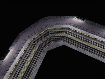
Fig. 6.3. A common 90 degrees bend in the On A Rail chapter in Half-Life. Shown in this figure is one such example in the map c2a2e. In an optimised speedrun, the player would be moving extremely fast in this section due to an earlier boost.

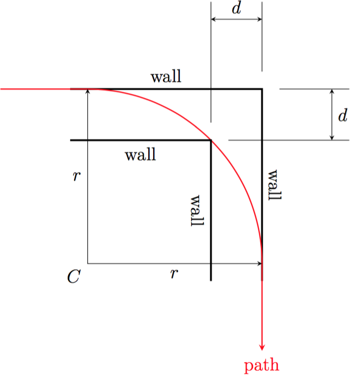
Fig. 6.4. Simplifying model of a common scenario similar to the one shown in Fig. 6.3..

We start by making some simplifying assumptions that will greatly reduce the difficulty of analysis while closely modelling actual situations in practice. Referring to Fig. 6.4., the first assumption we make is that the width of the corridor is the same before and after the turn. This width is denoted as 𝑑, as one can see in the figure. This assumption is justified because this is often true or approximately true in Half-Life maps. The second assumption is that the path is circular. The centre of this circle, also named the centre of curvature, is at point 𝐶. As noted earlier, the strafing path is in general a spiral with varying radius of curvature. Nevertheless, the total time required to make such a turn is typically very small. Within such short time frame, the radius would not have changed significantly. Therefore it is not absurd to assume that the radius of curvature is constant while making the turn. The third assumption is that the positions of the player before and after making the turn coincide with the walls. This assumption is arguably less realistic, but the resulting path is the larger circular arc one can fit in this space.

By trivial applications of the Pythagorean theorem, it can be shown that the relationship between the radius of curvature 𝑟 and the width of the corridor 𝑑 is given by

𝑟=(2+√2)𝑑≈3.414𝑑

This formula may be used to estimate the maximum radius of curvature for making such a turn without collision. However, the radius of curvature by itself is not very useful. We may wish to further estimate the maximum speed corresponding to this 𝑟.

6.6.2. Radius-speed relationship

The following figure depicts the positions of the player at times 𝑡 =0, 𝑡 =𝜏 and 𝑡 =2𝜏. The initial speed is ‖𝐯‖. All other symbols have their usual meaning.

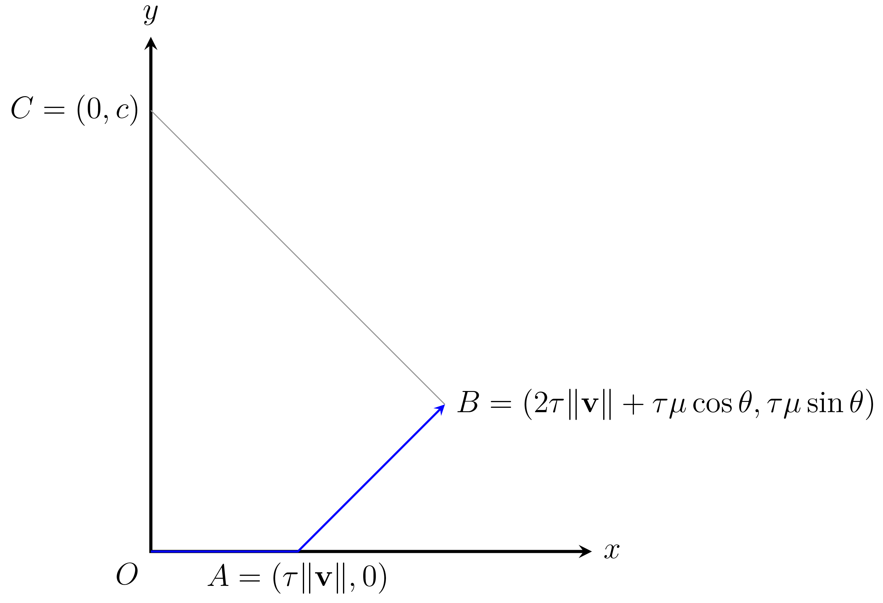
Based on the figure, the radius of curvature may be approximated as the 𝑦-intercept, or 𝑐. Obviously, a more accurate approximation may be achieved by averaging 𝑐 and BC. However, this results in a clumsy formula with little benefit. Empirically, the approximation by calculating 𝑐 is sufficiently accurate in practice. In consideration of this, it can be calculated that

(6.10)𝑟≈𝑐=𝜏sin⁡𝜃(2𝜇‖𝐯‖2+3‖𝐯‖cos⁡𝜃+𝜇)

Note that this is the most general formula, applicable to any type of strafing. From this equation, observe that the radius of curvature grows with the square of speed. This is a fairly rapid growth. On the other hand, under maximum speed strafing, the speed grows with the square root of time. Informally, the result of these two growth rates conspiring with one another is that the radius of curvature grows linearly with time. We also observe that the radius of curvature is directly influenced by 𝜏, as experienced strafers would expect. Namely, we can make sharper turns at higher frame rates.

From Equation (6.10) we can derive formulae for various types of strafing by eliminating 𝜃. For instance, in Type 2 strafing we have 𝜃 =𝜋/2. Substituting, we obtain a very simple expression for the radius:

𝑟≈𝜏(2𝐿‖𝐯‖2+𝐿)

Or, solving for ‖𝐯‖, we obtain a more useful equation:

‖𝐯‖≈√𝐿2(𝑟𝜏−𝐿)

For Type 1 strafing, the formula is clumsier. Recall that we have 𝜇 =𝑘𝑒𝜏𝑀𝐴 and

cos⁡𝜃=𝐿−𝑘𝑒𝜏𝑀𝐴‖𝐯‖

To eliminate sin⁡𝜃, we can trivially rewrite the cos⁡𝜃 equation in this form

sin⁡𝜃=√‖𝐯‖2−(𝐿−𝑘𝑒𝜏𝑀𝐴)2‖𝐯‖

Then we proceed by substituting, yielding

𝑟≈𝜏‖𝐯‖√‖𝐯‖2−(𝐿−𝑘𝑒𝜏𝑀𝐴)2(2𝑘𝑒𝜏𝑀𝐴‖𝐯‖2+3𝐿−2𝑘𝑒𝜏𝑀𝐴)

We cannot simplify this equation further. In fact, solving for ‖𝐯‖ is non-trivial as it requires finding a root to a relatively high order polynomial equation. As per the usual strategy when facing similar difficulties, we resort to iterative methods.